I am analyzing the complexity of different sorting and searching methods based on C programming language. To truly understand these methods, the author writes C programs to compare the performances of these methods based on large amounts of data generated randomly. The programs run several times, and the average amount of time used for each program is recorded and analyzed, compared to the theoretical amount of time from the textbooks. The results show that among the different sorting techniques, merge sort and shell sort based on Knuth’s sequence perform well. Large amounts of data can be well sorted in the AVL tree (or self-balancing binary search tree), since the height of the usual binary search tree may increase dramatically as the data increases. This study emphasizes the need to organize data, and to properly sort them in order to have them accessed easily. The author will continue his study by reading more books and running programs.
The author wishes to express sincere appreciation to Professors Yifu Cai for his assistance in the preparation. He is an excellent professor in physics and a leading researcher in the field of cosmology, and he taught me how to write papers properly. He shared his experiences as a professor and student, which encouraged me whenever faced with difficulties. In addition, special thanks to my senior students Jiarui Li, Qingqing Wang, and Xiaohan Ma for sharing your awesome research papers to me and offering me valuable advice during my research.
Part 1 Analysis of different sorting methods
Basics of an Algorithm
According to the book “An Introduction to Algorithms” by Thomas Cormen, "Informally, an algorithm is a well-defined computational procedure that takes some value, or sets of values, as input and produces some value, or set of values, as output.”
Thus, an algorithm is a sequence of computational steps that transform the input into the output. The algorithm describes a specific computational procedure for achieving that input/output relationship.
An algorithm is said to be correct if, for every input instance, it halts with the correct output.
Analysis of an Algorithm
The author analyzed his results mainly based on the complexity of time and space, and the best and worst case of his program, and the stability of each sorting technique.
Case analysis:
Worst-case: T(n) = maximum time of algorithm on any input of size n.
Average-case: T(n) = expected time of algorithm over all inputs of size n.
Best case: T(n) = minimum time of algorithm on any input of size n.
Here are a list of sorting methods the author used during his research
Insertion Sort
Insertion sort is a simple sorting algorithm that works like sorting the cards in your hand. The array is actually divided into sorted and unsorted parts. The value of the unsorted part is picked up and placed in the correct position in the sorted part.
Bubble Sort
Bubble Sort is also a simple and intuitive sorting algorithm. It repeatedly walks through the sequence to be sorted, comparing two elements at a time, and swapping them if they are in the wrong order. The work of visiting the sequence is repeated until no more exchanges are needed, that is, the sequence has been sorted. The name of this algorithm comes from the fact that the smaller elements are slowly "floated" to the top of the sequence by swapping.
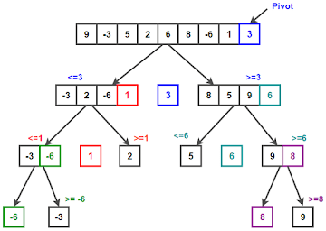
Quicksort
- Select one element at a time
- The elements larger than this element are arranged behind it, and the elements smaller than this element are arranged in front of it
- Algorithm complexity o(nlogn)
void quickSort(int arr[], int start, int end)
{

    // base case
    if (start >= end)
        return;

    // partitioning the array
    int p = partition(arr, start, end);

    // Sorting the left part
    quickSort(arr, start, p - 1);

    // Sorting the right part
    quickSort(arr, p + 1, end);

}
Overall, quicksort is the fastest sorting method
Graph: How quicksort works
Merge Sort
Main idea: Divide-and-conquer
- Divide the sequence into two until each group has only one element
- sort each set of arrays
- Merge each two sets of ordered series, if there are more than one series, continue to 2
Since each set of arrays is ordered, merging will be fast - Algorithm complexity o(nlogn)
Shell Sort
Shell sort is a generic version of the insertion sort algorithm. It sorts elements that are far apart first, and then sequentially reduces the spacing between the elements to be sorted. The spacing between elements decreases according to the order in which they are used.
int shellSort(int arr[], int n)
{
// Start with a big gap, then reduce the gap
for (int gap = n/2; gap > 0; gap /= 2)
{
// Do a gapped insertion sort for this gap size.
// The first gap elements a[0..gap-1] are already in gapped order

        for (int i = gap; i < n; i += 1)
        {
            // add a[i] to the elements that have been gap sorted
            // save a[i] in temp and make a hole at position i
            int temp = arr[i];

            // shift earlier gap-sorted elements up until the correct
            // location for a[i] is found
            int j;
            for (j = i; j >= gap && arr[j - gap] > temp; j -= gap)
                arr[j] = arr[j - gap];

            //  put temp (the original a[i]) in its correct location
            arr[j] = temp;
        }
    }
    return 0;

}
Knuth’s Sequence:
Donald Knuth invented a sequence to increase the efficiency of Shellsort. The sequence is this:
h = h * 3 + 1, where h is interval with initial value 1
This algorithm is quite efficient for medium-sized data sets as its average and worst-case complexity of this algorithm depends on the gap sequence the best known is Ο(n)
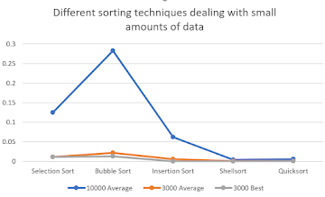
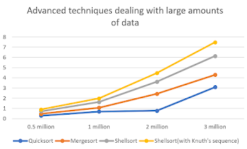
Then the author puts the time of the sorting techniques into an excel graph, which comes out like this
Note that though bucket sort can work extremely fast sometimes, it only work for data that can be listed as integers. For example, when sorting [13, 534, 46, 34, 52], bucket sort may work, however, when sorting float numbers, or doubles, bucket sort won’t work because it can’t put the data into the corresponding bucket, or arrays.
Summary
- Selection and bubble sorting are very slow
- Insertion sort is also slow, but when the array is sorted, it is very fast
- Quicksort and Hill sort has a speed of o(nlogn)
- The quick sort time is about 2 times the merge sort time, and the shellsort time is about 1.5 times the merge sort time
Algorithm Time Complexity
| Algorithm | Best | Average | Worst |
|---|---|---|---|
| Quicksort | Ω(n log(n)) | Θ(n log(n)) | O(n²) |
| Merge sort | Ω(n log(n)) | Θ(n log(n)) | O(n log(n)) |
| Bubble Sort | Ω(n) | Θ(n²) | O(n²) |
| Insertion Sort | Ω(n) | Θ(n²) | O(n²) |
| Selection Sort | Ω(n²) | Θ(n²) | O(n²) |
| Shell Sort | Ω(nlog(n)) | Θ((n(log(n))²) | O((n(log(n))²) |
| Bucket Sort | Ω(n+k) | Θ(n+k) | O(n²) |
Part 2: Searching in static array
Binary Search
One of the most important searching methods in Binary Search
The basic steps to perform Binary Search are:
- Begin with the mid element of the whole array as a search key.
If the value of the search key is equal to the item then return an index of the search key. - Or if the value of the search key is less than the item in the middle of
the interval, narrow the interval to the lower half. - Otherwise, narrow it to the upper half.
- Repeatedly check from the second point until the value is found or the interval is empty.
//binary search
asl=0;
for(j=0;j<avenum;j++)
{
    //i=1000*(rand()%(M/1000))+rand()%1000;//printf(\n%lld,i);
    i=rand()%M;
    key=a[i];num=0;left=0;right=M-1;
for(;left<=right;)
{
mid=(left+right)/2;
if(a[mid]==key){num++;break;}
else if(a[mid]>key){right=mid-1;num++;}
else{left=mid+1;num++;}
}
asl+=num;//printf(%5d%5d,asl,num);
}
printf(\n);
printf(\nexpected:%.3lf,(double)log(M+1)/log(2)-1);
left=0;right=M-1;
Fibonaccian Search
Similarities with Binary Search:
- Works for sorted arrays
- A Divide and Conquer Algorithm.
- Has Log n time complexity.
Differences with Binary Search:
- Fibonacci Search divides given array into unequal parts
- Binary Search uses a division operator to divide range. Fibonacci Search doesn’t use /, but uses + and -. The division operator may be costly on some CPUs.
- Fibonacci Search examines relatively closer elements in subsequent steps. So when the input array is big that cannot fit in CPU cache or even in RAM, Fibonacci Search can be useful.
//  fibonaccian search
int fib[40];
for(i=0;i<40;i++)
{
if(i==1||i==0)
{
fib[i]=i;
continue;
}
fib[i]=fib[i-1]+fib[i-2];
}
asl=0;
int k=0;
for(j=0;j<avenum;j++)
{
i=rand()%M;
    key=a[i];num=0;left=0;right=M-1;
    for(;left<=right;)
    {
    if(left==right||left==right-1)mid=left;
    else
    {
                for(k=0;;k++)
{
if(fib[k]>right-left+1)break;};mid=left+fib[k-2];}
if(a[mid]==key){num++;break;}
else if(a[mid]>key){right=mid-1;num++;}
else{left=mid+1;num++;}
}
    asl+=num;//printf(%5d%5d,asl,num);
}
printf(\n);
left=0;right=M-1;
Sequential Search
Sequential search is also known as serial or linear search. Searching an unordered list for a given data item is a very straightforward technique. The specified data items are searched sequentially in the list, that is, starting from the first data item, until the desired data item in the list.
Using sequential search, use the following process:
Compare the desired value with the first value of the list.
If the desired value matches the first value, declare the search operation successful and stop.
//  sequential search
asl=0;
for(j=0;j<avenum;j++)
{
//	i=1000*(rand()%(M/1000))+rand()%1000;//printf(\n%lld,i);
i=rand()%M;
asl+=(i+1);
}
printf(\n);
printf(\nexpected:%.3lf,(double)(M+1)/2);


//  interpolation search
asl=0;
for(j=0;j<avenum;j++)
{
    num=0;left=0;right=M-1;
//	i=1000*(rand()%(M/1000))+rand()%1000;//printf(\n%lld,i);
        i=rand()%M;


    key=a[i];
    for(;left<=right;)
    {
        if(left==right)mid=left;
        else{t=(key-a[left]);t=t*(right-left);
                                            t=t/(a[right]-a[left]);mid=left+t;}
        if(a[mid]==key)
        {
            num++;
            break;
        }
        else if(a[mid]>key)
        {
            right=mid-1;
            num++;
        }
        else
        {
            left=mid+1;
            num++;
        }
    }
//
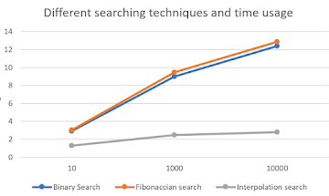
After running these programs, this graph is generated as a result of the various searching methods.
Hash Table
Hash Table is a data structure which stores data in an associative manner. In a hash table, data is stored in an array format, where each data value has its own unique index value. Access of data becomes very fast if we know the index of the desired data.
Donald Knuth analyzed address conflicts in his Art of Computer Programming and the results are as follows
α=(Records stored in the table)/(Maximum preset records in the table)
Linear detection method ASL=(1+1/(1-α))/2
Secondary detection method ASL=-ln〖(1−α)/α〗
Chain address method ASL=1+α/2
Part 3 Trees and Searching
Graph: a binary search tree
Binary Search Tree
Binary Search Tree is a node-based binary tree data structure which has the following properties:
- The left subtree of a node contains only nodes with keys lesser than the node’s key.
- The right subtree of a node contains only nodes with keys greater than the node’s key.
- The left and right subtree each must also be a binary search tree.
AVL Tree
Traversal
As a read-only operation the traversal of an AVL tree functions the same way as on any other binary tree. Exploring all n nodes of the tree visits each link exactly twice: one downward visit to enter the subtree rooted by that node, another visit upward to leave that node's subtree after having explored it.
Once a node has been found in an AVL tree, the next or previous node can be accessed in amortized constant time. Since there are n−1 links in any tree, the amortized cost is 2×(n−1)/n, or approximately 2.
void pre_order_traversal(struct node* root) {
   if(root != NULL) {
      printf(%d ,root->data);
      pre_order_traversal(root->leftChild);
      pre_order_traversal(root->rightChild);
   }
}


void inorder_traversal(struct node* root) {
   if(root != NULL) {
      inorder_traversal(root->leftChild);
      printf(%d ,root->data);
      inorder_traversal(root->rightChild);
   }
}


void post_order_traversal(struct node* root) {
   if(root != NULL) {
      post_order_traversal(root->leftChild);
      post_order_traversal(root->rightChild);
      printf(%d , root->data);
   }
}
Insert
NODE *create()
{
     NODE *newnode;
     int n;
     newnode=(NODE *)malloc(sizeof(NODE));
     printf(\n\nEnter the Data );
     scanf(%d,&n);
     newnode->data=n;
     newnode->llink=NULL;
     newnode->rlink=NULL;
     return(newnode);
}
void insert(NODE *root)
{
     NODE *newnode;
     if(root==NULL)
     {
          newnode=create();
          root=newnode;
     }
     else
     {
          newnode=create();
          while(1)
          {
               if(newnode->data<root->data)
               {
                    if(root->llink==NULL)
                    {
                         root->llink=newnode;
                         break;
                    }
                    root=root->llink;
               }
               if(newnode->data>root->data)
               {
                    if(root->rlink==NULL)
                    {
                         root->rlink=newnode;
                         break;
                    }
                    root=root->rlink;
               }
          }
     }
}